Master Excel Autofit: How to Instantly Resize Columns to Fit Your Data

Have you ever opened an Excel spreadsheet only to find a sea of frustrating ### errors, or text that awkwardly spills over into three neighboring columns? When you are dealing with large datasets, manual resizing is a massive waste of time.

Fortunately, Excel has a built-in feature called Autofit that instantly adjusts column widths to perfectly match the length of your longest data entry.

Here is your ultimate guide to mastering Autofit in Excel, featuring the quickest mouse shortcuts, ribbon methods, and keyboard combinations to clean up your sheets in seconds.

Method 1: The Double-Click Shortcut (The Fastest Way)

The absolute quickest way to fix a cramped column is by using a simple mouse shortcut.

1. Hover your mouse cursor over the right border of the column letter you want to fix (for example, the line between Column A and Column B).
2. Your cursor will transform from a thick white cross into a black double-sided arrow.
3. Double-click the mouse button.

Excel will instantly analyze the column and snap its width to fit the longest text or number inside it.

Pro Tip: Want to Autofit multiple columns at once? Click and drag across the column headers to highlight them all, then double-click the right border of any highlighted column. Every selected column will instantly resize to fit its respective data perfectly.

Method 2: The Excel Ribbon Route

If you prefer using the standard menu interface, or if you need to apply Autofit as part of a larger formatting routine, you can use the Excel Ribbon.

1. Select the columns you want to adjust (click the column letters at the top). If you want to apply this to the entire sheet, click the Select All triangle in the top-left corner where the row numbers and column letters meet.
2. Ensure you are on the Home tab at the top of the screen.
3. Look toward the right side of the ribbon and locate the Cells group.
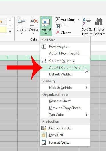
4. Click on the Format dropdown button.
5. Under the Cell Size section, click Autofit Column Width.

Method 3: The Power-User Keyboard Shortcuts

If you hate lifting your hands off the keyboard, you can execute an Autofit without touching your mouse. Excel offers sequential hotkeys that navigate the ribbon interface entirely via your keyboard.

First, select the column(s) you want to fix by using Ctrl + Space (which selects the entire current column). Then, type one of the following sequences depending on your operating system:

For Windows:

Press these keys one after another (do not hold them down together):

$$\text{Alt} \rightarrow \text{H} \rightarrow \text{O} \rightarrow \text{I}$$

• Alt activates the ribbon shortcuts.
• H selects the Home tab.
• O opens the Format menu.
• I triggers Autofit Column Width.

For Mac:

Mac users can use a more traditional combined shortcut. Select your columns and press:

$$\text{Control} + \text{Option} + \text{I}$$

Why Am I Still Seeing ### After Autofit?

Occasionally, you might trigger Autofit and still see a row of hashtags (###). This is Excel’s protective way of saying, “A number or date is too wide for this cell, and I refuse to cut it off and give you the wrong data.”

If Autofit doesn’t clear the ### error, it usually means your cell contains a number formatted with a specific text layout or a long date that requires slightly more breathing room than the default calculation provides. Simply click the column border and drag it slightly to the right to add a tiny bit of manual padding, and your numbers will reappear.